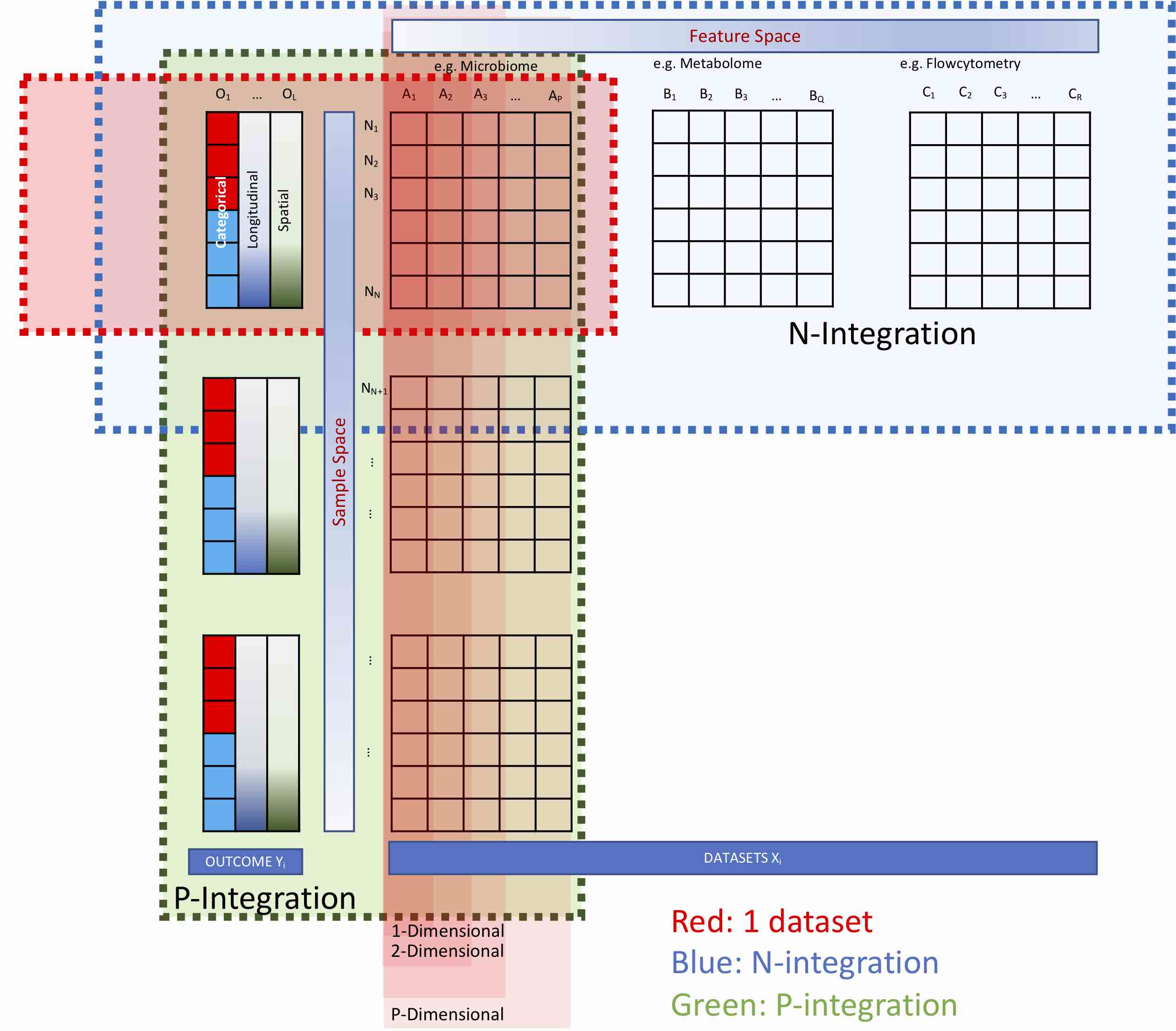
Pairwise Scenario
This section is referring to wiki page-4 of zone section-4 that is inherited from the zone section-7 by prime spin-5 and span- with the partitions as below.
(10 - 2) th prime = 8th prime = 19

f(8 twins) = 60 - 23 = 37 inner partitions
p r i m e s
1 0 0 0 0 0
2 1 0 0 0 1 ◄--- #29 ◄--- #61
3 2 0 1 0 2 👉 2
4 3 1 1 0 3 👉 89 -29 = 61 - 1 = 60 ✔️
5 5 2 1 0 5 👉 f(37) = f(8 twins) ✔️
6 7 3 1 0 7 ◄--- #23
7 11 4 1 0 11 ◄--- #19
8 13 5 1 0 13 ◄--- # 17 ◄--- #49
9 17 0 1 1 17 ◄--- 7th prime 👉 7s
10 19 1 1 1 ∆1 ◄--- 0th ∆prime ◄--- Fibonacci Index #18
-----
11 23 2 1 1 ∆2 ◄--- 1st ∆prime ◄--- Fibonacci Index #19 ◄--- #43
..
..
40 163 5 1 0 ∆31 ◄- 11th ∆prime ◄-- Fibonacci Index #29 👉 11
-----
41 167 0 1 1 ∆0
42 173 0 -1 1 ∆1
43 179 0 1 1 ∆2 ◄--- ∆∆1
44 181 1 1 1 ∆3 ◄--- ∆∆2 ◄--- 1st ∆∆prime ◄--- Fibonacci Index #30
..
..
100 521 0 -1 2 ∆59 ◄--- ∆∆17 ◄--- 7th ∆∆prime ◄--- Fibonacci Index #36  👉 7s
-----
Let weighted points be given in the plane . For each point a radius is given which is the expected ideal distance from this point to a new facility. We want to find the location of a new facility such that the sum of the weighted errors between the existing points and this new facility is minimized. This is in fact a nonconvex optimization problem. We show that the optimal solution lies in an extended rectangular hull of the existing points. Based on this finding then an efficient big square small square (BSSS) procedure is proposed.
Subclasses of Partitions
Integers can be considered either in themselves or as solutions to equations (Diophantine geometry).
Young diagrams associated to the partitions of the positive integers 1 through 8. They are arranged so that images under the reflection about the main diagonal of the square are conjugate partitions (Wikipedia).
f(8🪟8) = 1 + 7 + 29 = 37 inner partitions
p r i m e s
1 0 0 0 0 0
2 1 0 0 0 1 ◄--- #29 ◄--- #61
3 2 0 1 0 2 👉 2
4 3 1 1 0 3 👉 89 -29 = 61 - 1 = 60
5 5 2 1 0 5 👉 f(37) = f(8🪟8) ✔️
6 7 3 1 0 7 ◄--- #23
7 11 4 1 0 11 ◄--- #19
8 13 5 1 0 13 ◄--- # 17 ◄--- #49
9 17 0 1 1 17 ◄--- 7th prime 👉 7s
10 19 1 1 1 ∆1 ◄--- 0th ∆prime ◄--- Fibonacci Index #18
-----
11 23 2 1 1 ∆2 ◄--- 1st ∆prime ◄--- Fibonacci Index #19 ◄--- #43
..
..
40 163 5 1 0 ∆31 ◄- 11th ∆prime ◄-- Fibonacci Index #29 👉 11
-----
41 167 0 1 1 ∆0
42 173 0 -1 1 ∆1
43 179 0 1 1 ∆2 ◄--- ∆∆1
44 181 1 1 1 ∆3 ◄--- ∆∆2 ◄--- 1st ∆∆prime ◄--- Fibonacci Index #30
..
..
100 521 0 -1 2 ∆59 ◄--- ∆∆17 ◄--- 7th ∆∆prime ◄--- Fibonacci Index #36  👉 7s
-----
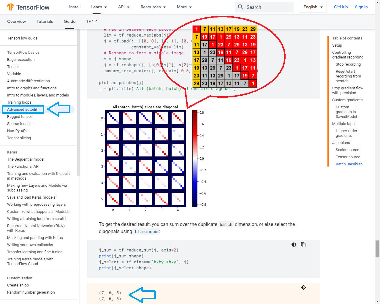
When these subclasses of partitions are flatten out into a matrix, you want to take the Jacobian of each of a stack of targets with respect to a stack of sources, where the Jacobians for each target-source pair are independent .
Feynman diagram for the same process as in the animation, with the individual quark constituents shown, to illustrate how the fundamental strong interaction gives rise to the nuclear force. Straight lines are quarks, while multi-colored loops are gluons (the carriers of the fundamental force). Other gluons, which bind together the proton, neutron, and pion “in-flight”, are not shown. The π⁰ pion contains an anti-quark, shown to travel in the opposite direction, as per the Feynman–Stueckelberg interpretation. (Wikipedia)

In summary, it has been shown that partitions into an even number of distinct parts and an odd number of distinct parts exactly cancel each other, producing null terms 0x^n, except if n is a generalized pentagonal number n=g_{k}=k(3k-1)/2}, in which case there is exactly one Ferrers diagram left over, producing a term (−1)kxn. But this is precisely what the right side of the identity says should happen, so we are finished. (Wikipedia)
p r i m e s
1 0 0 0 0 0
2 1 0 0 0 1 ◄--- #29 ◄--- #61
3 2 0 1 0 2 👉 2
4 3 1 1 0 3 👉 89 -29 = 61 - 1 = 60
5 5 2 1 0 5 👉 f(37) = f(29🪟23) ✔️
6 7 3 1 0 7 ◄--- #23
7 11 4 1 0 11 ◄--- #19
8 13 5 1 0 13 ◄--- # 17 ◄--- #49
9 17 0 1 1 17 ◄--- 7th prime 👉 7s
10 19 1 1 1 ∆1 ◄--- 0th ∆prime ◄--- Fibonacci Index #18
-----
11 23 2 1 1 ∆2 ◄--- 1st ∆prime ◄--- Fibonacci Index #19 ◄--- #43
..
..
40 163 5 1 0 ∆31 ◄- 11th ∆prime ◄-- Fibonacci Index #29 👉 11
-----
41 167 0 1 1 ∆0
42 173 0 -1 1 ∆1
43 179 0 1 1 ∆2 ◄--- ∆∆1
44 181 1 1 1 ∆3 ◄--- ∆∆2 ◄--- 1st ∆∆prime ◄--- Fibonacci Index #30
..
..
100 521 0 -1 2 ∆59 ◄--- ∆∆17 ◄--- 7th ∆∆prime ◄--- Fibonacci Index #36  👉 7s
-----
The code is interspersed with python, shell, perl, also demonstrates how multiple languages can be integrated seamlessly.
These include generating variants of their abundance profile, assigning taxonomy and finally generating a rooted phylogenetic tree.
p r i m e s
1 0 0 0 0 0
2 1 0 0 0 1 ◄--- #29 ◄--- #61
3 2 0 1 0 2 👉 2
4 3 1 1 0 3 👉 89 - 29 = 61 - 1 = 60
5 5 2 1 0 5 👉 f(37) = ❓ 👈 Composite ✔️
6 7 3 1 0 7 ◄--- #23
7 11 4 1 0 11 ◄--- #19
8 13 5 1 0 13 ◄--- # 17 ◄--- #49
9 17 0 1 1 17 ◄--- 7th prime 👉 7s 👈 Composite ✔️
10 19 1 1 1 ∆1 ◄--- 0th ∆prime ◄--- Fibonacci Index #18
-----
11 23 2 1 1 ∆2 ◄--- 1st ∆prime ◄--- Fibonacci Index #19 ◄--- #43
..
..
40 163 5 1 0 ∆31 ◄- 11th ∆prime ◄-- Fibonacci Index #29 👉 11
-----
41 167 0 1 1 ∆0
42 173 0 -1 1 ∆1
43 179 0 1 1 ∆2 ◄--- ∆∆1
44 181 1 1 1 ∆3 ◄--- ∆∆2 ◄--- 1st ∆∆prime ◄--- Fibonacci Index #30
..
..
100 521 0 -1 2 ∆59 ◄--- ∆∆17 ◄--- 7th ∆∆prime ◄--- Fibonacci Index #36  👉 7s
-----
This behaviour in a fundamental causal relation to the primes when the products are entered into the partitions system.
Composite behaviour
The subclasses of partitions systemically develops characters similar to the distribution of prime numbers. It would mean that there should be some undiscovered things hidden within the residual of the decimal values.
168 + 2 = 170 = (10+30)+60+70 = 40+60+70 = 40 + 60 + ∆(2~71)
p r i m e s
1 0 0 0 0 0
2 1 0 0 0 1 ◄--- #29 ◄--- #61
3 2 0 1 0 2 👉 2
4 3 1 1 0 3 👉 89 - 29 = 61 - 1 = 60
5 5 2 1 0 5 👉 f(37) ✔️
          6 👉 11s Composite Partition ✔️
6 7 3 1 0 7 ◄--- #23
7 11 4 1 0 11 ◄--- #19
8 13 5 1 0 13 ◄--- # 17 ◄--- #49
9 17 0 1 1 17 ◄--- 7th prime
           18 👉 7s Composite Partition ✔️
10 19 1 1 1 ∆1 ◄--- 0th ∆prime ◄--- Fibonacci Index #18
-----
11 23 2 1 1 ∆2 ◄--- 1st ∆prime ◄--- Fibonacci Index #19 ◄--- #43
..
..
40 163 5 1 0 ∆31 ◄- 11th ∆prime ◄-- Fibonacci Index #29 👉 11
-----
41 167 0 1 1 ∆0
42 173 0 -1 1 ∆1
43 179 0 1 1 ∆2 ◄--- ∆∆1
44 181 1 1 1 ∆3 ◄--- ∆∆2 ◄--- 1st ∆∆prime ◄--- Fibonacci Index #30
..
..
100 521 0 -1 2 ∆59 ◄--- ∆∆17 ◄--- 7th ∆∆prime ◄--- Fibonacci Index #36  👉 7s
-----
The initial concept of this work was the Partitioned Matrix of an even number w≥ 4:
- It was shown that for every even number w≥ 4 it is possible to establish a corresponding Partitioned Matrix with a determined number of lines.
- It was demonstrated that, fundamentally, the sum of the partitions is equal to the number of lines in the matrix: Lw = Cw + Gw + Mw.
- It was also shown that for each and every Partitioned Matrix of an even number w ≥ 4 it is observed that Gw = π(w) − (Lw − Cw), which means that the number of Goldbach partitions or partitions of prime numbers of an even number w ≥ 4 is given by the number of prime numbers up to w minus the number of available lines (Lwd) calculated as follows: Lwd = Lw − Cw.
To analyze the adequacy of the proposed formulas, probabilistically calculated reference values were adopted. (Partitions of even numbers - pdf)
p r i m e s
1 0 0 0 0 0
2 1 0 0 0 1 ◄--- #29 ◄--- #61
3 2 0 1 0 2 👉 2
4 3 1 1 0 3 👉 89 - 29 = 61 - 1 = 60
5 5 2 1 0 5 👉 11 + 29 = 37 + 3 = 40 ✔️
          6 👉 11s Composite Partition ◄--- 2+60+40 = 102 ✔️
6 7 3 1 0 7 ◄--- #23
7 11 4 1 0 11 ◄--- #19
8 13 5 1 0 13 ◄--- # 17 ◄--- #49
9 17 0 1 1 17 ◄--- 7th prime
           18 👉 7s Composite Partition
10 19 1 1 1 ∆1 ◄--- 0th ∆prime ◄--- Fibonacci Index #18
-----
11 23 2 1 1 ∆2 ◄--- 1st ∆prime ◄--- Fibonacci Index #19 ◄--- #43
..
..
40 163 5 1 0 ∆31 ◄- 11th ∆prime ◄-- Fibonacci Index #29 👉 11
-----
41 167 0 1 1 ∆0
42 173 0 -1 1 ∆1
43 179 0 1 1 ∆2 ◄--- ∆∆1
44 181 1 1 1 ∆3 ◄--- ∆∆2 ◄--- 1st ∆∆prime ◄--- Fibonacci Index #30
..
..
100 521 0 -1 2 ∆59 ◄--- ∆∆17 ◄--- 7th ∆∆prime ◄--- Fibonacci Index #36  👉 7s
-----
It’s possible to build a Hessian matrix for a Newton’s method step using the Jacobian method. You would first flatten out its axes into a matrix, and flatten out the gradient into a vector (Tensorflow).
(11x7) + (29+11) + (25+6) + (11+7) + 4 = 77+40+31+18+4 = 170